Osam Javed

Assignment 3 was all about ray tracing. It was definitely one of the most difficult and enjoyable projects that I've ever done. The project was setup well so that we could focus on the core concepts of ray tracing. From a high level of what I did in this project I, generated the camera rays, traced the ray for its spectrum radiance, implemented sphere and triangle ray intersection, accelerated our ray intersection by using a bounding volume hierarchy, casted shadow rays with a probability density function for direct and indirect illumination (used russian roulette in latter for unbiased random shadow ray termination), calculated the BSDF for mirrors and glass, used surface normal to get reflection, applied Snell's Law to enable refraction, and Schlick's approximation for the Fresnel factor to determine the specular reflection coefficient (using reflected or transmitted light).

Ray tracing creates such beautiful images because the lighting looks so realistic. However, in my 3 years of programming, I've never experienced 'waiting for my code', in this case to render highly sampled images. It felt like I was a programmer in the 80's waiting for my code to compile. My code is probably considerably slower than other pathtracers because my intersection code isn't optimized. I could make by BVH significantly faster if I used a better heuristic to handle the case where primitives aren't split evenly, as well as implementing a surface area heuristic. However even with all the optimizations that can currently be done for ray tracers, it's hard to imagine that ray tracing could be used for real time applications like gaming. This has led me to start thinking about alternative ways to render high quality images (they probably don't make sense). I'm hoping to keep working on this project after I submit it so that I can continue to learn more about ray tracing, implement some of the extra credit, and have fun.

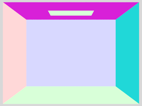
Part 1: Ray Generation and Intersection

As the title implies, part 1 really was all about ray genearation and scene intersection. The number of rays is passed in as an argument. I usually tested most of the early scenes with the sample rate set at 1, but used up to 1024 samples for high res images in parts 4 and 5. We generated the rays by calling the camera generate ray function. The camera generate ray function has a pinhole(viewpoint) which is positioned at the origin. The viewing window is our sensor plane which was one unit away from the pinhole. Given the two fields of view hFov and vFov, we defined our field of view from the pinhole to the viewing window. We used the gridSampler to get a uniformly random sample point in [0, 1] coordinates, and our input on the pixel space, we were able to determine the direction in camera space that the way would have to go. Before we passed in our random sample point + pixel space coordinates, we made sure to scale them down to [0, 1] coordinates by dividing by the sampleBuffer width and height of the pixel buffer. The idea is that for each pixel, we are calling random sample points on that individual pixels so we know where to shoot each ray on the pixel. To get the radiance of the pixel we call trace ray and average the spectrum values to return the color of that pixel in our final scene. The exception is that if we are sampling only one point on the pixel, then we would shoot the ray right in the middle of the pixel. To appropriately get the input point converted to a point on our viewing window, I did

(x, y) = (x*topRight.x + (1-x)*bottomLeft.x, y*topRight.y + (1-y)*bottomLeft.y)

This way, if the input was (0, 0) it would map to the bottom left of our viewing point, and (1, 1) would map to the top right of our viewing window. Since we want the ray going through our world coordinates, we convert the camera ray direction to the actual world coordinates by multiplying by cameraToWorldSpace. Getting all this camera and world conversion is really important or else the direction we cast our rays will be totaly off. We now had the rays origin, direction, and the rays intersection t values were provided with information of the camera in nClip being the rays defualt min_t value and fClip the rays default max_t value. Knowing a ray's origin, intersection times, and direction, meant that I could finally shoot off my rays. The next step was implementing triangle and sphere intersection since both objects were returning false by default.

To implement triangle intersection, I implemented the Moller Trumbone algorithm. One of the advantages of triangles is that they belong to a single plane, we can define them to be in xy, xz, yz. Using barycentric coordinates, we know that if a ray intersects a triangle, it does so at one or between two vertices. We parametize as a ray in this region with an intersection point P. The cool thing about barycentric coordinates is that they give us an idea of the 'center of mass' for a triangle. With this defined, it doesn't matter if our triangle is scaled or rotated. The area proportions of the triangle will remain consistent. To define barycentric coordinates all we needed were coordinates u and v, to enable ray intersection, MT also takes into account t (distance until intersection from ray origin to triangle). MT finds these 3 unknown t,u,v values by applying Cramer's rule which solves a system of linear equations (t, u, v). If we have a system of 3 linear equations, we can express the coefficiets in a M = 3x3 matrix, the RHS of this system is represented as a column vector, C. We want to find another column vector C' = (x, y, z) such that M * C' = C. Finding C' is done evaluating the determinant of M, Mx, My, Mz where Mx is M but with the first column replaced by C, M_y second column C and same for Mz. The cool thing about Cramer's law is that it helps find the determinant of our matrix M with the following equations:

 Input: Matrix M, Mx, My, Mz, C.  Output: C' column vector * M = C.
			  x = Mx/M, y=My/M, z=Mz/M

Now that we have found C', we can find the determinant of a 3x3 matrix M by using a triple scalar product which is similar to finding the determinant of a 1x3 column vector. Once we have t, u, v. Using the determinant, MT determines how our ray intersects with a triangle. f the determinant is less than 0, the triangle is backfacing, if it equals 0 then our ray didn't hit our triangle (ray shot in parallel to our triangle, doesn't hit its face). What the determinant is really doing here is giving us a consistent way to define the position of our triangle so that we have a defined normal vector N coming out of the face of our triangle. We can now define if we hit our triangle from the top, bottom, side depending on the determinant value. Sphere intersection was much more simple. We know that our ray can hit our sphere at either 1 (tangent to sphere) or 2 hits. To determine whether our ray hit the sphere (or a solution exists) we see if a solution for a quadratic exists by checking if the discriminant is greater than 0. If so, we know there was an intersection. We updated our ray's max_t value with the new distance it took to first have an intersection with our sphere. I think the reason for this is that it really optimizes our code. Once we know a ray intersects an object closer to the pinhole, there's no need to check for any intersections behind the object (since the viewer won't see there). The object closest to the pinhole is the most important.

Some of the bugs I had in raytrace_pixel in part 1 didn't haunt me until later parts of the project. I was confused why I couldn't sample at 1 pixel and needed 4 pixels to see anything. This bug happened to be that in my for loop I was sampling the center of the pixel for the first sample, and not terminating if the number of samples requested was 1. Sadly, I generated a ray but did not use the return value when I traced the ray. (Explained why my renderings were all black!). When there was only 1 sample per pixel, I also wasn't scaling down to [0, 1] coordinates for the camera_generate_ray function. In my sphere intersection, I wasn't checking the ray intersection t bounds, and was also improperly always setting t1 as the max_t.

No sphere intersection

Spheres with normal shading

Nicely colored dragon

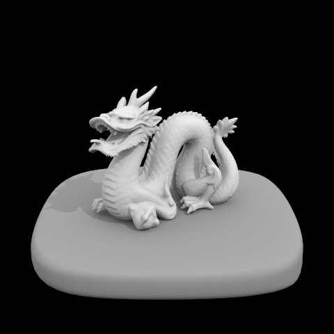
Part 2: Bounding Volume Hierarchy

I used a recursive algorithm to construct my BVH. It could have been more memory efficient if I used a stack and iterative algorithm. Once the bounding and centroid box had been created for all the primitives, I would see which axis of the bounding box was the largest. I compared the bounding box's extent on the x, y, z axis. My split point along this axis would then be the midpoint of the axis, easily found by using the centroid_box.centroid() function. Since the centroid was a vector 3D, I would access the axis that I found to be the largest in the bbox extent earlier. Once I had a split point, I would create two vector lists called left and right and add every primitive to the left of my split point in the left vector, else add to the right vector. The primitive location could be found by its centroid method as well. Once I had the left and right vector list populated, I would construct another sub-BVH and recursively do this until there were at most max_leaf_size amount of primitives remaining in each BVH. Over spring break, my program was seg faulting because I couldn't properly implement how to handle one of the cases where one of my vector lists contained no primitives. My main idea was that if one of the vector lists was empty, I would get one item from the other vector list and insert it into the emtpy vector. This way the recursion wouldn't continue on an empty vector.

My BVH intersection algorithm was pretty simple. I first had to implement the bounding_box intersection function. This is probably the messiest function I have in the entire project. Given a ray and the t intersection times I would determine if an intersection that occured is valid. I first made sure that all the t0 times were less than t1 else I would swap them. Then I would ensure that the min time for an axis wasn't greater than the max time for another axis, or else that would be an invalid intersection and I would return false. In order to speed up my BVH, I tried to return false on as many condiitons as possible before returning a valid intersection. I would reset the min and max intersection t time according to the max of min t axis values, and the min of the max t values. This ensured that I had the tightest t_min and t_max ray bounds on my bounding box. As long as there was a common intersection between all axis', and the final t_min was less than the t_max, would I then finally return True for a valid BBox intersection. Once the BBox intersection was complete, the BVH intersection was simple as it defined on the BBox intersection entirely. If the ray didn't intersect a bounding box, I would immediately return false. Else I would check if that node is a leaf (where primitives actually exist), and if the ray intersected with any primitive in that BBox, would I return true. I recursively called my BVH intersect until a leaf node with limited primitives was found.

I think not having a BVH and being unable to render many of images in part1, made me appreciate BVH construction so much more. Implementing BVH made my code order of magnitudes faster (linear to log). Even though I was handling the case of an empty left/right vector poorly, most of the BVH construction would happen in a matter of seconds. I know that my BVH would be much faster if I sorted primitives by their centroid location and transferred half the primitives to the empty list vector. But I was having some trouble with the C++ comparator function. My heuristic in some cases probably makes my BVH run in linear time as I'm eventually just handing off one primitive at a time to the empty vector. I'm going to try to fix this soon, but overall the BVH is still running super fast. Implementing the surface area hueristic seems like a fun optimization I'll experiment with.

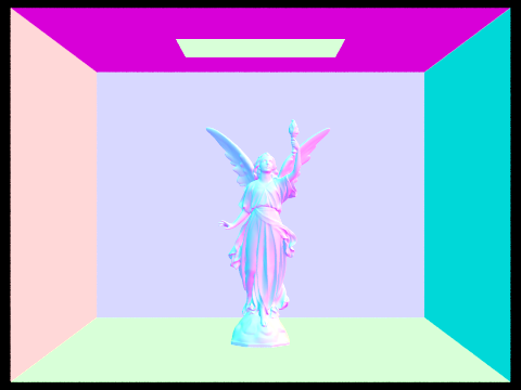
Lucy and her million triangles required a BVH model to render

Finally saw Maxplanck's face after implementing BVH.

Part 3: Direction Illumination

In part3, luckily a lot of the object to world space conversion was done for us. In my implementation I took samples from every light source in the scene and would calculate the BSDF of that surface using the radiance sampled. A delta function is a function that's zero every except at zero. We had delta lights in our scenes which meant that it would only be necessary to sample these light sources at one location. However for all the lights that weren't constrained to a delta function, we needed to sample over ns_area_lights. This light parameter is what we passed in as program arguments depending on how many light sources we wanted to sample with. I would get a light sample by calling the sample_L function with the distance to light and probability density function variables to be filled in. Using this light sample, I would calculate the BSDF by getting the light towards the direction of the ray w_i, convert it to object space -> w_in, cast a shadow ray to see if it intersect with my BVH. If it did I would accumulate the light coming out of this surface in L_out. Here is where I used the BSDF of the surface and the light sample to get the amount of lighting at the surface. To ensure that there was no bias toward certain regions of the light source, I would divide by the pdf returned at that sampled light location.

I was getting a lot of speckels in my scene during part 3 because my ray was not able to get off the ground. (Intersecting with the ground resulted in lots of black spots). Once I was able to figure out the ray was getting stuck, I offset the ray's min_t value by 0.01 to ensure it had enough runway for takeoff :) Although, this problem is most likely due to some floating point precision failure. Another thing I did wrong was instead of creating a spectrum for the sampled light, I would accumulate the sampled light in my L_out variable.

Direct illumination seen on chest, foreground, and background.

Direct darker shadow underneath dragon, lighter shadow on foreground

Bunny sampled with 1 sample/area light.

Bunny sampled with 2 sample/area light. Not a huge difference.

Bunny sampled with 4 sample/area light. Here we can notice how the light shadow casted in the foreground of the bunny is more detailed and stronger.

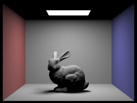
Part 4: Indirect Illumination

Part 4 was cool because we used Russian roulette as an unbiased way to determine the BSDF on our surface. The probability of a shadow ray surviving was the bsdf of the surface multiplied by the illumination from that spot. I multiplied the surviaval probability by 10 to make sure the rays weren't cut off too short (avoiding the black speckle problem). However, I used the C++ clamp function to ensure that the probability remained between [0, 1]. The coin flip function took in our ray survivial probability and determined whether or not to cast a shadow ray. This shadow ray's origin was again offset by EPS_D to ensure we weren't sampling the same region of the light source repeatedly. The incoming radiance was determined by calling the trace_ray function which evaluates the radiance at our shadowRay's hitpoint. To make sure that we have unbiased sampling, I divided by the pdf and probability of our ray survival.

I think the most challenging part of Indirect Illumination was implementing the idea of using Russian Roulette correctly to cast shadow rays with unbiased light sampling. I was originally offsetting my ray by just EPS_D resulting in a speckeled image, but later multiplied by o2w * w_in. Also, my lambertians were getting very odd shading from misplaced normals because I wasn't multiplying by the abs(w_in.z).

Results Caption: my bunny is the bounciest bunny

Here is an example of how to include a simple formula:

a^2 + b^2 = c^2

or, alternatively, you can include an SVG image of a LaTex formula.

This time it's your job to copy-paste in the rest of the sections :)

Part 5: Materials

Implementing reflect was pretty easy as I used what I did in the last project, I created my normal vector with it set at the origin and the z axis at 1. I then took the dot product between the cosine term and multiplied by 2 * (normal - light out). To calculate the BSDF on mirror materials, I set the pdf to 1, since perfect mirrors don't lose light. I would then call the BSDF reflect function, and return the amount of reflected light divided by the cosine of the incoming light. Refract was a very tricky BSDF to calculate since refraction depends on the medium which it refracts through. I used Snell's law to determine whether the light should refract. If the cosine term was less than 0, I would swap the refractive indices. I would return the total internal reflection if sin theta 0 less than 1.0 which is my n0 value. To calculate the glassBSDF, if the light didn't refract I would return the amount of reflected light divided by the cos of the incoming light. Else if the light did refract, I used Schlick's approximation to get the reflection coefficient from the Fresnel equations. Using the algorithm provided on the spec, I used the reflection coefficient as a probability to whether there was reflection or refraction. If it reflected I would use the amount fo reflected light, else the amount of transmitted light.

Luckily the algorithm for glass BSDF was given so I didn't have too many errors for that part. Luckily, refract wasn't too horrible for me as many people seemed to struggle on it, so there was a lot of help on Piazza to help guide me through. It was so interesting to see how different materials respond differently to the amount of light given. I really appreciate how well mirrors reflect light now!